Starting and running your first Notebook

Setup

Open up a Terminal and do the following steps:

  • change directory to CS157
  • make new directory, call it something like Notebooks (for example: mkdir Notebooks)
  • change directory to your newly created directory
  • issue the command conda init bash and if it asks any yes or no questions, just hit return
  • issue the command conda activate to set up your environment to run our data science frameworks
  • issue the command jupyter notebook to start up the server

This last starts up a Jupyter server and will automatically start your web browser if it wasn't already running. The server is what executes the things you run in the notegbook.


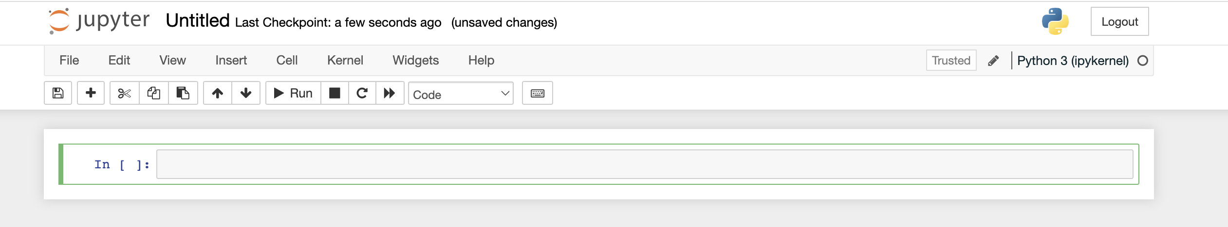
Creating the first Notebook page

The Jupyter Home Page is ready for you start creating. You should see something like this, but without all the files:
alt text

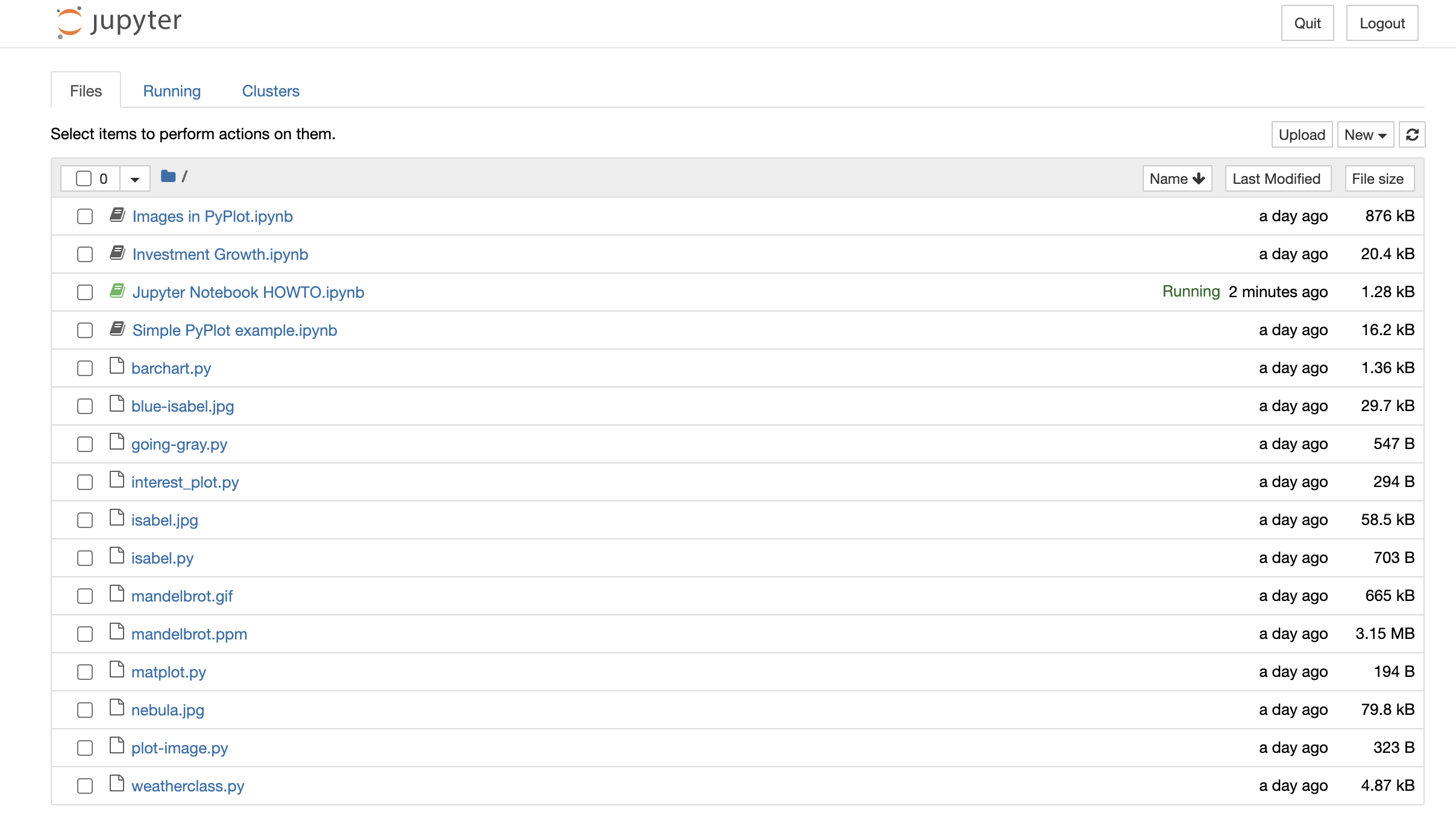
Click the New button near the upper right hand corner to begin a new Notebook page. It's a pull-down menu; generally we'll want a Python3 page but notice that you can create a text file, a new directory, or even open an online Terminal (try it and see...later).

Your new page looks something like:
alt text

A few cosmetic things to get started:

  • Click on the text Untitled at the top and rename with an actual title for your page (note: the title will also be used to name the notebook when saved)
  • From the pull-down menu which says Code select Markdown
  • In the first cell (labeled In [ ]:) type ## My First Notebook, then type Shift-Enter (shift key and enter key together)

Now your page will look like this

altText

For more about the formatting you can do in Markdown cells, see this bit or this other bit

Run a Python script

Now to make sure of the setup, run some Python. Copy the script below into a code cell and execute by simply typing Shift-Enter:

import matplotlib.pyplot as plt

princ = 10000
int_rate = 0.05
years = 20
values = []

for _ in range(years+1):
    values.append(princ)
    princ += princ*int_rate

plt.plot(values)
plt.title('5% Growth')
plt.xlabel('Years of Compounding')
plt.ylabel('Value of Principlal ($)')

If you get a proper graph from that, terrific. Now to complete the task, save the Notebook page, then go to the File menu, select Download As and pick HTML. You can save this HTML version of the file in the same directory the notebook is in. Now in the browser you can do File -> Open File... and load the HTML version of your notebook into the browser as a static web page. Demonstrate this page to the instructor.

We'll talk about how HTML files go on our webserver later.

Shutting down Jupyter

To finish up, click the Logout button in the upper right hand corner. You can now close the tab. Go back to the tab labeled Home Page and click the Quit button. Then just to be sure, change back to the Terminal window where you started the Jupyter notebook server to begin with; typing Ctrl-C twice should shut down the server. Finally, to leave the Data Science virtual environment, issue the command conda deactivate.

In [ ]: